This is the thirty fifth part of the ILP series. For your convenience you can find other parts in the table of contents in Part 1 – Boolean algebra
Last time we saw how to implement Special ordered sets in ILP. Today we are going to use this knowledge to implement piecewise linear approximation in one dimension and in two dimensions. Let’s start.
Table of Contents
Idea
Let’s take simple non-linear function ![]() . We already know how to multiply numbers in ILP but representing
. We already know how to multiply numbers in ILP but representing ![]() in this way might be computationally intensive and hence we would like to avoid this kind of formulation. However, if we don’t need to be 100% precise it might be better to approximate this function if we know the possible range of
in this way might be computationally intensive and hence we would like to avoid this kind of formulation. However, if we don’t need to be 100% precise it might be better to approximate this function if we know the possible range of ![]() . Let’s assume that we have these points:
. Let’s assume that we have these points:
![]()
we are now able to calculate the following values:
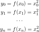
So for every known argument we simply calculate the function ![]() . If all
. If all ![]() are integers this looks very trivial, however, if
are integers this looks very trivial, however, if ![]() are reals and
are reals and ![]() is a bit more complicated then precalculating the function value might greatly simplify the ILP model for our problem.
is a bit more complicated then precalculating the function value might greatly simplify the ILP model for our problem.
Having all these points, we declare variable representing actual argument:
![]()
So we define ![]() as real number in range
as real number in range ![]() , which we will use as an argument of function
, which we will use as an argument of function ![]() . However, instead of simply calculating
. However, instead of simply calculating ![]() we will approximate it using linear functions in ranges
we will approximate it using linear functions in ranges ![]() .
.
1D Approximation
We will use the following trick: for all linear functions we define “weights” of vertices and use them to approximate function. They are defined in the following manner:
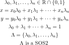
Introduced lambda variables guarantee that ![]() will lie in one of the segments
will lie in one of the segments ![]() thanks to SOS2 constraints. Without this stipulation would allow the
thanks to SOS2 constraints. Without this stipulation would allow the ![]() variable to “lie” on other segments, probably ranging over multiple
variable to “lie” on other segments, probably ranging over multiple ![]() variables. The same goes for
variables. The same goes for ![]() variable — by using lambda variables we are able to approximate
variable — by using lambda variables we are able to approximate ![]() correctly.
correctly.
Let’s consider an example: ![]() with function
with function ![]() and values
and values ![]() . We have the following relation:
. We have the following relation:

And now imagine that ![]() , we get
, we get ![]() and
and ![]() which is quite a good approximation. However, if it happens that
which is quite a good approximation. However, if it happens that ![]() is on a grid (which we can force by making
is on a grid (which we can force by making ![]() binary variables), we get exact solution.
binary variables), we get exact solution.
Our approximated value is represented by variable ![]() so in the remaining part of our ILP model we use
so in the remaining part of our ILP model we use ![]() in place of
in place of ![]() .
.
2D Approximation
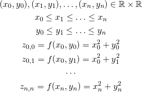
Approximation in two dimensions goes almost exactly the same. We have the function ![]() and the following points:
and the following points:
We introduce the following variables:
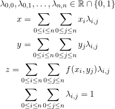
We now need to add constraint similar to SOS2 for 1D approximation. In that case the constraint simply meant “at most two neighbouring variables are allowed to be non-zero”. Now we need to add constraint “at most four neighbouring variables are allowed to be non-zero” which is simply a generalization of SOS2 (bonus chatter: you might guess how to approximate 3D function). We introduce the following variables:
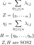
If we allow lambdas to be real numbers (e.g., we don’t require ![]() and
and ![]() to lay on a grid), we need to make sure that non-zero lambda variables lay on a triangle. We can do that by introducing another SOS2 set:
to lay on a grid), we need to make sure that non-zero lambda variables lay on a triangle. We can do that by introducing another SOS2 set:

Summary
We know how to approximate 1D and 2D functions using special ordered sets of type 2. By using this approach we can greatly reduce size of ILP models which might significantly decrease solving time.