This is the eleventh part of the ILP series. For your convenience you can find other parts in the table of contents in Part 1 – Boolean algebra
Last time we implemented a selection sort in ILP. Today we are going to do something similar: we are going to implement counting sort.
Table of Contents
Introduction
As you probably remember from your classes, counting sort is useful when we try to sort values from small and finite set. It is for instance great for sorting people by their age because there are no people older than 200 years so we have at most two hundred possible values (and we can confine this range even more). What’s more, counting sort time complexity is linear so in theory it should work faster than selection sort. So let’s begin.
Problem definition
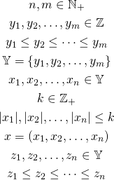
First, let’s define necessary variables:

We have ![]() variables
variables ![]() to sort. Every
to sort. Every ![]() variable has a value from set
variable has a value from set ![]() . Set
. Set ![]() has
has ![]() variables
variables ![]() . Variables
. Variables ![]() represents the final result.
represents the final result.
We are going to sort variables ![]() using the knowledge that they all come from the set
using the knowledge that they all come from the set ![]() .
.
Algorithm
Our algorithm will have the following steps:
- Compare every
 with every
- Sum results of comparisons to know how many values are there actually
- Construct the final vector
Comparing
We define the following variables:
![]()
We basically try to find them number of values ![]() in vector
in vector ![]() . After this step we have
. After this step we have ![]() different variables.
different variables.
Summing results
Now we need to know how many values are there so we define the following variables:
![Rendered by QuickLaTeX.com \[ c_{y_i} = \sum_{j=1}^{n} c_{y_i = x_j} \]](../../../../wp-content/ql-cache/quicklatex.com-525da98e32b50744803dcde8de09bf77_l3.png)
Now we know that there are exactly ![]() values
values ![]() in vector
in vector ![]() . We now need to aggregate the results to be able to reconstruct the vector, so we define the partial sums:
. We now need to aggregate the results to be able to reconstruct the vector, so we define the partial sums:
![Rendered by QuickLaTeX.com \[ s_{i} = \sum_{j=1}^{i} c_{y_i} \]](../../../../wp-content/ql-cache/quicklatex.com-2c0ed077af0bae9e00889b1728553997_l3.png)
This value tells us that there are exactly ![]() elements not greater than
elements not greater than ![]() . This might be a bit tricky so let’s consider an example first.
. This might be a bit tricky so let’s consider an example first.
Example
Let’s imagine that we want to sort the following vector:
![]()
We can see that ![]() and we have
and we have ![]() values. We also assume the following set of possible values:
values. We also assume the following set of possible values:
![]()
Basically we assumed that our values are not greater than ![]() and not less than
and not less than ![]() . It is worth noting that in
. It is worth noting that in ![]() there is no variables equal to
there is no variables equal to ![]() but this is how counting sort works. We now have the following results of comparisons:
but this is how counting sort works. We now have the following results of comparisons:

Now we need to aggregate these values:

Right now we know that there are exactly ![]() variables in vector
variables in vector ![]() equal to
equal to ![]() . Now we sum the results:
. Now we sum the results:

And now we know that there are exactly ![]() values not greater than
values not greater than ![]() in vector
in vector ![]() ,
, ![]() values not greater than
values not greater than ![]() and so on.
and so on.
Constructing the result
Every ![]() variable tells us how many values not greater than
variable tells us how many values not greater than ![]() there are in the original vector. We can utilize this knowledge to put values in correct places:
there are in the original vector. We can utilize this knowledge to put values in correct places:
![]()
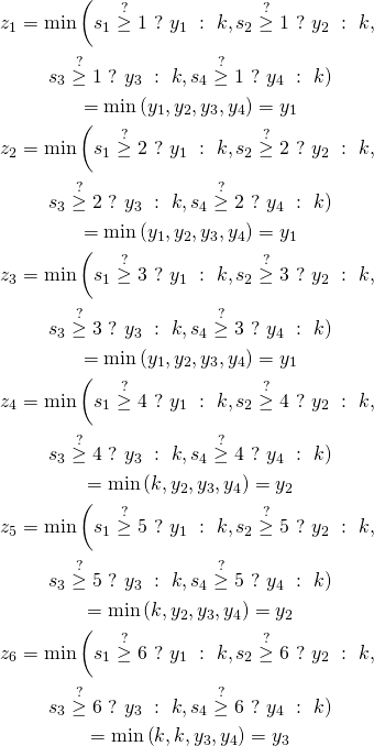
In our example it is:

This works in the following way: for every position ![]() we ask whether there are at least
we ask whether there are at least ![]() elements not greater than
elements not greater than ![]() and we choose minimum of
and we choose minimum of ![]() values. So we basically try to insert values in their places and we need to use
values. So we basically try to insert values in their places and we need to use ![]() function to select lowest possible value for every place.
function to select lowest possible value for every place.
Complexity
As you can see, this algorithm needs ![]() temporary variables. Assuming that
temporary variables. Assuming that ![]() our algorithm uses linear space. If it is not true that
our algorithm uses linear space. If it is not true that ![]() then it makes no sense using this algorithm but the same happens with casual counting sort. There is no use to sort numbers using this algorithm when the domain is really big.
then it makes no sense using this algorithm but the same happens with casual counting sort. There is no use to sort numbers using this algorithm when the domain is really big.
Summary
We already know two sorting algorithms. Their implementation is rather straightforward and really resembles the imperative counterparts. As an exercise you might want to implement other imperative algorithms using similar approach.