This is the sixtieth fourth part of the ILP series. For your convenience you can find other parts in the table of contents in Part 1 – Boolean algebra
Last time we actually implemented BFS-like algorithm in the graph with ILP which can be also used for testing graph connectivity (if two nodes are connected transitively) or building any spanning tree. Today a simplified and clear solution for the BFS in ILP. We take this graph:
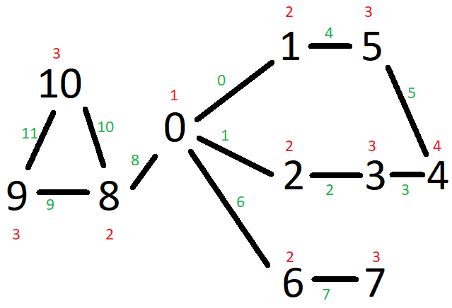
Black numbers represent nodes. Green numbers represent edge identifiers (we number edges for simplicity). Red numbers are calculated distances increased by one (to differentiate between no distance and calculated distance, so between zero and one).
The code:
|
1 2 3 4 5 6 7 8 9 10 11 12 13 14 15 16 17 18 19 20 21 22 23 24 25 26 27 28 29 30 31 32 33 34 35 36 37 38 39 40 41 42 43 44 45 46 47 48 49 50 51 52 53 54 55 56 57 58 59 60 61 62 63 64 65 66 67 68 69 70 71 72 73 74 75 76 77 78 79 80 81 82 83 84 85 86 87 88 89 90 91 92 93 94 95 96 97 98 99 100 101 102 103 104 105 106 107 108 109 |
var solver = new CplexMilpSolver(10); var edgeEnds = new Tuple<int, int>[]{ Tuple.Create(0, 1), Tuple.Create(0, 2), Tuple.Create(2,3), Tuple.Create(3,4), Tuple.Create(1,5), Tuple.Create(4,5), Tuple.Create(0,6), Tuple.Create(6,7), Tuple.Create(0,8), Tuple.Create(8,9), Tuple.Create(8,10), Tuple.Create(9,10) }; var board = Enumerable.Range(0, edgeEnds.SelectMany(t => new int[]{t.Item1, t.Item2}).Max() + 1).Select(n => edgeEnds.Where(t => t.Item1 == n || t.Item2 == n).Select(t => t.Item1 == n ? t.Item2 : t.Item1).ToArray()).ToArray(); Console.WriteLine("Create variables"); var nodes = Enumerable.Range(0, board.Length).Select(c => new System.Dynamic.ExpandoObject()).ToArray(); for(int node=0;node<nodes.Length;++node){ dynamic self = nodes[node]; self.Identifier = solver.CreateAnonymous(Domain.PositiveOrZeroInteger); self.Degree = solver.CreateAnonymous(Domain.PositiveOrZeroInteger); self.IsStart = solver.CreateAnonymous(Domain.BinaryInteger); self.LowerNeighboursCount = solver.FromConstant(0); } var edges = Enumerable.Range(0, board.SelectMany(e => e).Max() + 1).Select(c => new System.Dynamic.ExpandoObject()).ToArray(); for(int edge=0;edge<edges.Length;++edge){ dynamic self = edges[edge]; self.InPath = solver.CreateAnonymous(Domain.BinaryInteger); } Console.WriteLine("Set starting point (optional)"); solver.Set(ConstraintType.Equal, solver.FromConstant(1), ((dynamic)nodes[0]).IsStart); Console.WriteLine("Calculate degree"); for(int node=0;node<nodes.Length;++node){ dynamic self = nodes[node]; var neighbours = board[node].Select(i => edges[i]).Select(e => (IVariable)((dynamic)e).InPath).ToArray(); solver.Set(ConstraintType.Equal, self.Degree, solver.Operation(OperationType.Addition, neighbours)); } Console.WriteLine("Make exactly one starting point"); solver.Set(ConstraintType.Equal, solver.FromConstant(1), solver.Operation(OperationType.Addition, nodes.Select(n => (IVariable)((dynamic)n).IsStart).ToArray())); Console.WriteLine("Make sure all nodes have positive degree"); for(int node=0;node<nodes.Length;++node){ dynamic self = nodes[node]; solver.Set(ConstraintType.GreaterOrEqual, self.Degree, solver.FromConstant(1)); } Console.WriteLine("Make sure neighbours differ by one"); for(int edge = 0; edge < edges.Length;++edge){ dynamic self = nodes[edgeEnds[edge].Item1]; dynamic other = nodes[edgeEnds[edge].Item2]; dynamic connection = edges[edge]; solver.Set(ConstraintType.Equal, solver.FromConstant(1), solver.Operation(OperationType.MaterialImplication, connection.InPath, solver.Operation(OperationType.IsEqual, solver.FromConstant(1), solver.Operation(OperationType.AbsoluteValue, solver.Operation(OperationType.Subtraction, self.Identifier, other.Identifier))))); } Console.WriteLine("Points on path have non-empty identifier"); for(int node=0;node<nodes.Length;++node){ dynamic self = nodes[node]; solver.Set(ConstraintType.GreaterOrEqual, self.Identifier, solver.FromConstant(1)); } Console.WriteLine("Calculate lower neighbours"); for(int edge = 0; edge < edges.Length;++edge){ dynamic self = nodes[edgeEnds[edge].Item1]; dynamic other = nodes[edgeEnds[edge].Item2]; dynamic connection = edges[edge]; self.LowerNeighboursCount = solver.Operation(OperationType.Addition, self.LowerNeighboursCount, solver.Operation(OperationType.Conjunction, connection.InPath, solver.Operation(OperationType.IsGreaterThan, self.Identifier, other.Identifier))); other.LowerNeighboursCount = solver.Operation(OperationType.Addition, other.LowerNeighboursCount, solver.Operation(OperationType.Conjunction, connection.InPath, solver.Operation(OperationType.IsGreaterThan, other.Identifier, self.Identifier))); } Console.WriteLine("Starting point has no lower neighours"); for(int node=0;node<nodes.Length;++node){ dynamic self = nodes[node]; solver.Set(ConstraintType.Equal, solver.FromConstant(1), solver.Operation(OperationType.MaterialImplication, self.IsStart, solver.Operation(OperationType.IsEqual, solver.FromConstant(0), self.LowerNeighboursCount))); } Console.WriteLine("Inner point has one lower neighbour"); for(int node=0;node<nodes.Length;++node){ dynamic self = nodes[node]; solver.Set(ConstraintType.Equal, solver.FromConstant(1), solver.Operation(OperationType.MaterialImplication, solver.Operation(OperationType.BinaryNegation, self.IsStart), solver.Operation(OperationType.IsEqual, solver.FromConstant(1), self.LowerNeighboursCount))); } var goal = solver.Operation(OperationType.Addition, nodes.Select(n => (IVariable)((dynamic)n).Identifier).ToArray()); solver.AddGoal("Goal", solver.Operation(OperationType.Negation, goal)); solver.Solve(); for(int node=0;node<nodes.Length;++node){ dynamic self = nodes[node]; Console.WriteLine(node + " - " + solver.GetValue(self.Identifier)); } |
We do the same thing as last time but let’s walk through it again.
First, in lines 3-16 we describe our graph. We specify edges by their ending nodes so for instance line 5 says there is an edge between node zero and node two. Next, in line 18 we transform this to an adjacency list for simplicity.
Next, in lines 20-29 we define variables for nodes. Each node has an identifier (distance from the source), degree (how many edges from the spanning tree it is connected to), flag whether this node is a BFS source, and a number of lower neighbours (neighbours with lower distance to the source).
In lines 31-36 we define variables for edges. Each edge can be included in the path (in the spanning tree) or not.
Finally, we can specify the BFS root in line 38-39 (if needed). That wraps the data preparation, now let’s build constraints.
In lines 41-47 we calculate degrees. For each node we take edges ending in the node and then check if they are included in the spanning tree.
In line 50 we make sure there is one starting point in the graph.
In lines 52-57 we make sure all nodes have positive degree so all of them are included in the spanning tree.
Next, we start building the BFS. In lines 59-66 we specify that distance must increase by one for each node (so neighbours differ by one).
In lines 68-73 we specify that each node has some distance calculated.
In lines 75-84 we count lower neighoburs for each node. We then use this value in lines 86-91 to specify that the BFS root has no lower neighbours (it has the lowest distance) and that inner nodes (lines 93-98) have exactly one lower neighbour (to avoid loops).
Now the crucial part for BFS: in lines 101-102 we sum the identifiers and minimize the result. This is to make sure all nodes have shortest path in graph with loops. If your graph has no loops (is a tree) then you don’t need this constraint as there is exactly one path between all node pairs. Obviously, it’s not required for connectivity so don’t use it if you don’t care about the distnaces.
Finally, we print the solution. It looks like this:
|
1 2 3 4 5 6 7 8 9 10 11 12 13 14 15 16 17 18 19 20 21 22 23 24 25 26 27 28 29 30 31 32 33 34 35 36 37 38 39 40 41 42 43 44 45 46 47 48 |
Tried aggregator 3 times. MIP Presolve eliminated 510 rows and 287 columns. MIP Presolve modified 326 coefficients. Aggregator did 114 substitutions. Reduced MIP has 159 rows, 94 columns, and 475 nonzeros. Reduced MIP has 77 binaries, 17 generals, 0 SOSs, and 0 indicators. Presolve time = 0.00 sec. (1.54 ticks) Probing fixed 0 vars, tightened 5 bounds. Probing time = 0.00 sec. (0.24 ticks) Tried aggregator 1 time. Reduced MIP has 159 rows, 94 columns, and 475 nonzeros. Reduced MIP has 77 binaries, 17 generals, 0 SOSs, and 0 indicators. Presolve time = 0.00 sec. (0.22 ticks) Probing fixed 0 vars, tightened 3 bounds. Probing time = 0.00 sec. (0.25 ticks) Clique table members: 364. MIP emphasis: balance optimality and feasibility. MIP search method: dynamic search. Parallel mode: deterministic, using up to 4 threads. Root relaxation solution time = 0.00 sec. (0.34 ticks) Nodes Cuts/ Node Left Objective IInf Best Integer Best Bound ItCnt Gap 0 0 0.0000 23 0.0000 33 * 0+ 0 0.0000 0.0000 33 0.00% 0 0 cutoff 0.0000 0.0000 33 0.00% Elapsed time = 0.02 sec. (3.67 ticks, tree = 0.00 MB, solutions = 1) Root node processing (before b&c): Real time = 0.02 sec. (3.68 ticks) Parallel b&c, 4 threads: Real time = 0.00 sec. (0.00 ticks) Sync time (average) = 0.00 sec. Wait time (average) = 0.00 sec. ------------ Total (root+branch&cut) = 0.02 sec. (3.68 ticks) 0 - 1 1 - 2 2 - 2 3 - 3 4 - 4 5 - 3 6 - 2 7 - 3 8 - 2 9 - 3 10 - 3 |
You can check that it matches red numbers in the picture.
Obviously, you can generalize this algorithm same way we did last time to match your needs. However, it is generic enough to be used to build continuous paths between nodes.