This is the first part of the Machine Learning series. For your convenience you can find other parts using the links below (or by guessing the address):
Part 1 — Linear regression in MXNet
Part 2 — Linear regression in SQL
Part 3 — Linear regression in SQL revisited
Part 4 — Linear regression in T-SQL
Part 5 — Linear regression
Part 6 — Matrix multiplication in SQL
Part 7 — Forward propagation in neural net in SQL
Part 8 — Backpropagation in neural net in SQL

In this series I assume you do know basics of machine learning. I will provide some source code for different use cases but no extensive explanation. Let’s go.

Today we will take a look at linear regression in MXNet. We will predict sepal length in well know iris dataset.

I assume you have the dataset uploaded to s3. Let’s go with loading the dataset:

from mxnet import nd, autograd
import pandas as pd
import matplotlib.pyplot as plt
from sklearn.model_selection import train_test_split

local_file="/tmp/Iris.csv"
df = pd.read_csv("/blabla/" + local_file, delimiter=',', header = 0)

print df.shape

from mxnet import nd, autograd

import pandas as pd

import matplotlib.pyplot as plt

from sklearn.model_selection import train_test_split

local_file="/tmp/Iris.csv"

df = pd.read_csv("/blabla/" + local_file, delimiter=',', header = 0)

print df.shape

We can see some records with print df.head(3) or check different iris categories with df.iris.unique().

We have one target variable and four features. Let’s create two adttional:

df['i_setosa'] = 0
df.loc[(df['iris']=='setosa'), 'i_setosa']= 1
df['i_versicolor'] = 0
df.loc[(df['iris']=='versicolor'), 'i_versicolor']= 1

df['i_setosa'] = 0

df.loc[(df['iris']=='setosa'), 'i_setosa']= 1

df['i_versicolor'] = 0

df.loc[(df['iris']=='versicolor'), 'i_versicolor']= 1

Two features similar to one hot encoding of categorical feature.

Time to prepare training and test datasets with: df_train, df_test = train_test_split( df, test_size=0.3, random_state=1)

Let’s get down to training. We start with defining the training variables and the target one:

independent_var = ['sepal_width','petal_length','petal_width','i_setosa','i_versicolor']
y_train = nd.array(df_train['sepal_length'])
X_train = nd.array(df_train[independent_var]) 
y_test = nd.array(df_test['sepal_length'])
X_test = nd.array(df_test[independent_var])

independent_var = ['sepal_width','petal_length','petal_width','i_setosa','i_versicolor']

y_train = nd.array(df_train['sepal_length'])

X_train = nd.array(df_train[independent_var])

y_test = nd.array(df_test['sepal_length'])

X_test = nd.array(df_test[independent_var])

Let’s prepare class representing data instance:

class data:
    def __init__(self,X,y):
        self.X = nd.array(X) 
        self.y = nd.array(y)
        cols = X.shape[1]
        self.initialize_parameter(cols)

    def initialize_parameter(self,cols):
        self.w = nd.random.normal(shape = [cols, 1])
        self.b = nd.random.normal(shape = 1)
        self.params = [self.w, self.b]

        for x in self.params:
            x.attach_grad()

class data:

def __init__(self,X,y):

self.X = nd.array(X)

self.y = nd.array(y)

cols = X.shape[1]

self.initialize_parameter(cols)

def initialize_parameter(self,cols):

self.w = nd.random.normal(shape = [cols, 1])

self.b = nd.random.normal(shape = 1)

self.params = [self.w, self.b]

for x in self.params:

x.attach_grad()

We initialize parameters and attach gradient calculation. This is a very nice feature, we don’t need to take care of derivatives, everything is taken care for us.

Let’s now carry on with a single step for gradient:

class optimizer:
    def __init__(self):
        pass
    
    def GD(self,data_instance,lr):
        for x in data_instance.params:
            x[:] = x - x.grad * lr

class optimizer:

def __init__(self):

pass

def GD(self,data_instance,lr):

for x in data_instance.params:

x[:] = x - x.grad * lr

We just subtract gradient multiplied by learning rate. Also, we use x[:] instead of x to avoid reinitializing the gradient. If we go with the latter, we will see the following error:

Check failed: !AGInfo::IsNone(*i) Cannot differentiate node because it is not in a computational graph. You need to set is_recording to true or use autograd.record() to save computational graphs for backward. If you want to differentiate the same graph twice, you need to pass retain_graph=True to backward.

Check failed: !AGInfo::IsNone(*i) Cannot differentiate node because it is not in a computational graph. You need to set is_recording to true or use autograd.record() to save computational graphs for backward. If you want to differentiate the same graph twice, you need to pass retain_graph=True to backward.

Now, let’s train our model:

def main():
    # Modeling parameters
    learning_rate = 1e-2
    num_iters = 100
    
    data_instance = data(X_train,y_train) 

    opt = optimizer()
    gd = optimizer.GD
    
    loss_sequence = []
    
    for iteration in range(num_iters):
        with autograd.record():
            loss = nd.mean((nd.dot(X_train, data_instance.w) + data_instance.b - y_train)**2)
            
        loss.backward()
        gd(opt, data_instance, learning_rate)
        
        print ("iteration %s, Mean loss: %s" % (iteration,loss))
        loss_sequence.append(loss.asscalar())
        
    plt.figure(num=None,figsize=(8, 6))
    plt.plot(loss_sequence)
    plt.xlabel('iteration',fontsize=14)
    plt.ylabel('Mean loss',fontsize=14)

def main():

# Modeling parameters

learning_rate = 1e-2

num_iters = 100

data_instance = data(X_train,y_train)

opt = optimizer()

gd = optimizer.GD

loss_sequence = []

for iteration in range(num_iters):

with autograd.record():

loss = nd.mean((nd.dot(X_train, data_instance.w) + data_instance.b - y_train)**2)

loss.backward()

gd(opt, data_instance, learning_rate)

print ("iteration %s, Mean loss: %s" % (iteration,loss))

loss_sequence.append(loss.asscalar())

plt.figure(num=None,figsize=(8, 6))

plt.plot(loss_sequence)

plt.xlabel('iteration',fontsize=14)

plt.ylabel('Mean loss',fontsize=14)

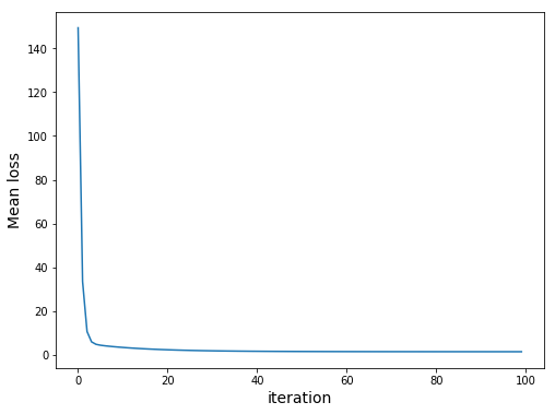
We should get the following:

Training - mean

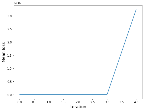
Note that our loss uses mean whereas we could calculate just a sum. However, due to overflow problems we would get the following:

Training - sum

Finally, let’s check the performance of trained model:

MSE = nd.mean(((nd.dot(X_test, data_instance.w) + data_instance.b) - y_test)**2)
print ("Mean Squared Error on Test Set: %s" % (MSE))

1 2	MSE = nd.mean(((nd.dot(X_test, data_instance.w) + data_instance.b) - y_test)**2) print ("Mean Squared Error on Test Set: %s" % (MSE))

Done.

Summary

We can see that linear regression is pretty concise and easy. However, this uses Python and Spark which me might want to avoid. In next parts we will take a look at different solutions.